Why emerging economies are (un)successful in avoiding the middle income trap

In the transition from an emerging market to an industrialised economy, India and China will have to avoid the so-called ‘middle income trap’. The middle income trap refers to the phenomenon that GDP per capita growth falls significantly after a certain threshold is reached, as wages start to rise and an emerging economy loses its comparative cost advantage (see Eichengreen et al., 2013). This threshold lies between USD 12,000 and USD 18,000 per capita (2015 purchasing power parities).[1]

Boosting labour productivity is key to avoid the middle income trap. There are examples of countries that have been successful in avoiding the middle income trap by transforming their economy: Singapore, Hong Kong, South Korea, Japan, Taiwan and Ireland.

A key transformation in these countries was that labour productivity was less and less driven by investment, but was gradually taken over by a high contribution of so-called total factor productivity[2] to growth. In contrast, other countries have been less successful, e.g. Brazil, Mexico, Indonesia and Thailand.

In this Special report we use a panel model for a specific set of countries which have started from a low income level and achieved considerable growth rates over time, but either got stuck in the middle income trap or were successful in avoiding it. We use modern panel estimation techniques to determine the factors that have been important in the (un)successful transformation of countries and subsequently use this model to run a number of scenarios for China and India. These two countries will determine the face of global growth and it is essential that these economic giants won’t be trapped in the middle income trap.

[1] The threshold by Eichengreen et al. (2013) lies between 10,000USD and 15,000USD, measured in 2005 PPP.

[2] Total factor productivity (TFP) is the part of economic growth which cannot be attributed to either more labour or capital inputs. Hence, TFP is an indicator of the efficiently of an economy.

There are several factors that are important in order to boost labour productivity and avoid the middle income trap. First, Eichengreen et al. (2013) find that developing high-quality human capital reduces the probability of a slowdown in growth. Korea is a prime example of a country where investment in secondary and tertiary education has helped to continue to boost growth. Second, Eichengreen et al. (2013) also conclude that a large share of high-tech exports is negatively associated with the likelihood of a slowdown. The result by Eichengreen et al. (2013) that innovative activity is an important factor to boost growth is confirmed by several other studies. For instance, Erken et al. (2016), Griffith et al. (2004), Engelbrecht (1997), Bassanini and Scarpetta (2002) and Cameron et al. (2005) all find a positive relationship between domestic technological capital and human capital on the one hand and productivity on the other hand. The average years of (tertiary) education is an indicator often used to measure the amount of human capital in a country (see Barro and Lee, 2013). This indicator is useful, although a disadvantage is that it does not take into account the quality level of education. Next to human capital, knowledge developed abroad is an important factor for productivity development (e.g. Coe and Helpman, 1995; Cohen and Levinthal, 1989; Erken et al., 2016). The idea is that countries with a relatively low level of technological development can benefit from knowledge developed elsewhere by using it in their own products or production processes. Through a process of so-called catching-up, low technological countries can narrow the gap in productivity with the technologically more advanced countries. There is a debate in the literature about the transmission channel of international knowledge spillovers, being either trade (Coe and Helpman, 1995; Grossman and Helpman, 1991) or foreign direct investments (Branstetter, 2006). Some studies argue that international spillovers are not driven by trade flows (Keller, 1998; Kao et al., 1999). We follow Branstetter (2006) and use FDI as a conduit of knowledge spillovers. A fourth factor that is important to avoid the middle income trap is the institutional quality of a country. In the literature, there is some debate about the causality between the institutional context and economic performance: do institutions themselves result in better economic performance, or does economic prosperity result in better institutions? In line with Bruinshoofd (2016), Coe et al. (2009) and Acemoglu and Robertson (2013), we build on the intuition that institutional development is an indicator for structural development and long-term welfare creation for a nation. Economic growth is therefore key for determining the short-term trajectory of a nation, almost regardless of its origin, but institutional development determines whether short-term gains are sustainable over the longer term. As such, high-quality institutions provides the environment for economic convergence and development, and allows countries to achieve long-term income convergence. There is also substantial empirical evidence in the literature that the institutional quality has a beneficial effect on the development of productivity and growth. In contrast to Coe et al. (2009), we adopt the view that a better score on institutional indicators also generates direct productivity benefits. For instance, better regulation lowers administrative burdens and X-inefficiencies[3] and allow people to be more productive in the amount of hours that they are working. Or a higher degree of openness to international trade will result in a more effective distribution of labour and, consequently, a more productive sector composition, which will be prosperous for productivity. Finally, we add two labour market variables as controls: the participation rate measured by the number of people engaged in work as a percentage of total population and, secondly, the number hours worked per person engaged in work. Both variables should have a negative impact on the development of productivity (see Belorgey et al., 2006; Bourlès and Cette, 2007; Erken et al., 2016). High labour participation is often characterized by increased deployment of less-productive labour, which lowers labour productivity. Working fewer hours may have a positive impact on productivity if less fatigue occurs among workers or if employees work harder during the shorter number of active hours.

[3] The term X-inefficiencies refers to slack in the production process and higher production costs than necessary, which are the result of lack of competitiveness pressure in the market.

The starting point for our framework is the human capital-augmented Solow model as introduced by Mankiw et al. (1992):

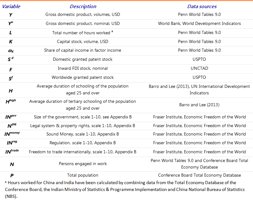
where Y denotes gross domestic product, K and L denote (physical) capital input and labor (measured in physical units such as hours worked) respectively. Furtermore, H represents human capital and A represents the level of (labor-augmented) technological change. Equation (1) can be transformed into:

If we take into account a varying output elasticity of capital, we arrive at the following equation:

where i is country, t is year and c is a constant term. The variables in equation (3) and their data sources are discussed in Table 1. The construction of patent capital is explained in Appendix A. All variables are expressed as an index (2000 = 1). The term related to α₁ measures the effect of the domestic patent stock per 100,000 persons engaged in work. Term α₂ is our knowledge catching-up variables, which picks up the effect of worldwide foreign patent capital per 100,000 persons engaged in work worldwide and is interacted with the foreign direct investment stock as a ratio of nominal GDP. FDI serves as a conduit to reap the productivity benefits of worldwide produced knowledge. Term α₃ represents human capital, α₄ and α₅ measure the effect of higher labour market activity and α₆ measures the effect of institutional variables.

Country selection

In order to select the proper countries for our sample, we use three criteria:

1. We exclude countries that have had a GDP per capita exceeding 10,000 USD PPP (measured in 2015 prices) in 1960. We use data from the Conference Board (Total Economy Database) to make this assessment. By applying this restriction, we exclude all industrialized countries, as well as the rich ones that rely solely on commodity exports. The latter ones haven’t had the urge to transform the economy in order to avoid the middle income trap, such as Saudi Arabia and the United Arab Emirates. For some countries, we don’t have any readings of GDP per capita in 1960.
2. The second selection criteria is that countries need to have had a computed annual growth rate (CAGR) between 1960 and 2000 of 2% or more. If time series do not start in 1960, we will examine the CAGR covering the period up till 2005. This way, we eliminate low-income countries that have hardly shown any economic progression over time, many of which are countries on the African continent.
3. Data availability on all drivers of labour productivity, i.e. hours worked, the capital stock, technological and human capital and data on institutional quality.

Ultimately, we estimate equation (3) for a panel of 23 countries over a time period covering 1970-2015. The countries are Barbados, Brazil, China, Costa Rica, Cyprus, Greece, Hong Kong, India, Ireland, Israel, Japan, Malaysia, Malta, Mexico, Poland, Portugal, Singapore, South Korea, Spain, Sri Lanka, Taiwan, Trinidad & Tobago, and Turkey.

Running regressions between time series with a long temporal component is hazardous, as there is a risk of obtaining spurious or nonsense correlations (Granger and Newbold, 1974). Especially levels data over time tends to be trended over time. An Augmented Dickey-Fuller is the useful test to examine if variables are stationary or not. In our case, key variables such as TFP and the patent stock, are non-stationary. Taking first differences of variables is usually sufficient to avoid the risk of running spurious results, but the downside is that we also lose much relevant information about long-term relationships. Especially the variance of institutional data tends to be rather constant over time and fails to show any relevance forn productivity when included in a first differences equation. However, taking first differences is not necessary if a particular combination of nonstationary variables exists that is stationary. In this case, non-stationary variables are said to be cointegrated (Engle and Granger, 1987). OLS estimates of cointegrated time series converge to their coefficient values much faster than in the case of stationary variables, making these regressions ‘super consistent’ (Greene 2000, p. 795).

Kao et al. (1999) argues that OLS estimations of non-stationary panel data will generate biased results, but dynamic ordinary least squares estimates (DOLS) estimation techniques are valid. DOLS uses cross-section-specific lags and leads of the differenced independent variables, which corrects for regressor endogeneity and serially correlated errors (Stock and Watson, 1993).

Our DOLS estimator has the following form:

where y_i,t is our dependent variable for country i and year t, x'_i,t is our matrix of independent variables, ϐ is our cointegration vector, i.e., the long-run cointegrated effect of our set of independent variables on our dependent variable, and υ is the error term.

Cointegration tests

Engle and Granger (1987) have developed tests to examine if variables are cointegrated: I(0). If variables are not cointegrated, then the residuals will be I(1). Kao (1999) also made the tests of Engle and Granger suitable for panel data analyses[4]. Table 2 shows the results of the cointegration tests. The results show that, regardless the number of variables used, the panel cointegration test rejects the null hypothesis of no cointegration. The only exception is when the institutional intellectual IPR variable is added (IN^IPR), the test is only statistically significant at 90%. These results imply that we can use dynamic ordinary least squares (DOLS) to estimate long-run relationships.

[4] We do not report the Phillips-Perron (PP) test and PP rho test, as these tests perform less well in finite samples than ADF tests (Davidson and MacKinnon, 2004, p. 623).

In column (1) in Table 3 we only include technological capital (c₁) and international knowledge spillovers (c₂) as two drivers of TFP. Both determinants have a significant positive effect and the magnitude of domestic knowledge capital is comparable to effects found in the literature (e.g. Coe et al., 2009, Kao et al., 1999). If we add human capital (c₃) in column (2), measured by the average years of schooling, the effects of domestic technological capital and technological catching-up remain robust, although the magnitude of the coefficients are somewhat lower. The coefficient of 0.37 for human capital is in line with effects found in the literature (e.g. Bassanini and Scarpetta, 2002; Erken et al., 2016). In the estimation shown in column (3), the control variable hours worked per person engaged (c₄) has the expected sign, although the magnitude is somewhat larger than estimations by Belorgey et al. (2006) and Bourlès and Cette (2007). This could be due to the estimation techniques, as Erken et al. (2016) have conducted DOLS for a panel of 20 OECD countries and found coefficients for hours worked exceeding the effects found by Belorgey et al. (2006) and Bourlès and Cette (2007) as well. The effect of participation (c₅) has a counter-intuitive sign and is insignificant. This differs from effects found in the literature (ibidem), which could be due to the fact that participation levels in our panel of countries is still significantly below the rates in OECD countries. We leave out this control variable in the rest of our estimations. In columns (5) to (9), we separately add one institutional variable to the baseline model. The effect of government size (c₆) and sound money (c₈) has the expected sign, but is insignificant. The effect of the legal system and property rights (c₇) has a significant negative effect, which is surprising. This outcome could be defended from an economic standpoint, as in an emerging market with high levels of intellectual property protection and enforcement knowledge spillovers are hampered, which consequently, would deter TFP development. However, as Table 2 shows, the set of variables are not cointegrating properly as well, which makes the outcome even more suspicious. We choose not to use this variable. Finally, column (8) and (9) show that regulatory quality (c₉) and freedom to trade internationally (c₁₀) have a significant and positive effect on TFP. However, the trade variable eats away the significance of our human capital variable. Therefore, we follow Eichengreen et al. (2013) and use the average level tertiary education as an alternative indicator for human capital. Our final model in column (10) shows positive and expected signs of all included variables and has the highest explanatory power. The estimated equation in column (10) will serve as our final model for running scenario analyses in the next section.

In this section, we will calculate the labour productivity effects in three different scenarios for India and China up till 2025. With these scenarios we aim to get a better feeling of the growth potential if China and India would foster technological capital (scenario 1), human capital (scenario 2), institutional quality (scenario 3). The assumptions for each scenario are elaborated on in Appendix C. We wrap up this section by looking at an extreme scenario in which India and China would be able to close the gap with the Asian top tier countries in the field of innovation, education and institutional quality.

The first step is to use the estimated model in Table 3 (column (10)) to produce TFP growth forecasts. Figure 2 and 3 illustrates the results of our baseline scenario and the scenarios. Indian TFP in the baseline would increase to 1.8% per annum in 2025, which is equal to the average annual growth rate over the entire observation period (1970-2015). Chinese TFP growth would amount to 1.4% per annum in 2025, which is somewhat less than the average (1.9%). If we accumulate the effects of all three scenarios on TFP growth, the full stimulus package would results in cumulative TFP gains which are equal to 25% in China in 2025 and 23% in India.

Although figures 2 and 3 suggest otherwise, it is important to stress that improvements on the determinants of productivity (technological capital, human capital and institutions) do not result in permanent higher TFP growth rates[5]. This is in line with the semi-endogenous growth theory of Jones (1995). If, for instance, the level of patent intensity would lead to higher growth rates, in line with insights from the growth theory by Young (1998), TFP growth would become unsustainably high. See for an extensive comparison of endogenous growth theories Donselaar (2011).

[5] The reason TFP appears to be boosted to permanent higher growth rates in 2025 is due to the fact that growth in patent capital is gradually increased up till a maximum in 2025. However, if we would remain all levels constant in the time frame after 2025, TFP growth would decline to the baseline level.

Labour productivity

As the TFP gains measured as an index is hard to interpret, we use the outcome from our scenario analyses to calculate a productivity outlook, of which TFP is one of the components. In order to do this, however, we also need a forecast structural capital deepening. For China, the largest contribution to labour productivity came from investment in non-ICT capital. After the meltdown of the global economy in 2008, the Chinese government has facilitated lending to the corporate sector in order to prop up private investment. Although this has helped to mitigate the negative effects of the Great Recession, it has also resulted in a surge of private debt-to-GDP ratios from 110% in 2008 to more than 200% in 2015. Moreover, additional lending to the corporate sector no longer seems to be having any positive effect on economic growth (see Erken and Kalf, 2016). This is partly explained by the fact that a large proportion of new lending is used to roll-over the existing large debt of Chinese state-owned enterprises (SOEs). Meanwhile, net profitability of these SOE’s is under pressure, which makes it more difficult for these firms to service their debt. Payment problems are mainly concentrated in more traditional industrial sectors that have a lot of overcapacity, such as coal and steel. We expect the high levels of capital deepening of the last decade to gradually decline over time (see Appendix D). For India, we expect capital deepening to be stable around 4.5%. We use four ARIMA models to extrapolate both the total amount of hours worked in India and China, as well as capital investment. Figure A.9 in the Appendix D illustrates our expectations of the growth contribution of capital deepening to structural labour productivity.

The translation to labour productivity for China is shown in Figure 4. In our baseline, labour productivity growth would gradually decline from 6.5% in 2014 to 3.5% in 2025. If we add the additional TFP contributions from our scenarios, the declining productivity in China would be mitigated to a large extent and growth would continue to hover around 6%. In 2025, half of total productivity growth would be the result of the stimulus of technological capital, human capital and improved institutional quality. Ultimately, Chinese labour productivity levels per hour would rise from roughly 11 USD in 2016 to almost 20 USD in 2025, which is 3.7 USD more than in the baseline. This has tremendous wealth effects, as it would add 6.5trn USD to the Chinese economy (3.7 USD times 1770bn hours). This is one-third of gross domestic product of the US in 2016 ($PPP, 2015 constant prices).

In India, the impetus would result in a upward growth trajectory (Figure 5), as we expect stable productivity growth in our baseline. In 2025, the level of productivity per hour would increase from 7.5 USD to 12.5 USD, 2.4 USD more than the baseline in 2025. This is equivalent to 3.1trn USD (2.4 times 1265bn hours) of additional gains for the Indian economy.

Reaching for the top

If China and India would be able to improve innovation, human capital and institutional quality to the front-runners in our country sample, the results would change drastically. This scenario would imply raising relative patenting levels to that of Taiwan (500 per 100,000 persons employed), boosting tertiary education to levels of South Korea (1.5 years of average tertiary education). Finally, the institutional framework would be changed to the standards of Hong Kong (freedom of trade = 9.4; quality of regulation = 9.0).

In this extreme scenario, labour productivity per hour in China would go up to 27 USD and in India to somewhat less than 15 USD (Figure 6 and 7). This is equivalent to 19trn USD of additional value added in China and 6trn in India.

The Chinese and Indian economy will determine the face of global growth in the years to come. In their slow transition from an emerging market to an industrialized economy, both economic giants will have to overcome the so-called ‘middle income trap’. This means that growth of an economy shifts to a lower gear, as a certain level of income is reached. Growth in emerging markets is often resource-driven, dependent on cheap labour and capital growth. When wages start to rise, the emerging economy loses its comparative cost advantage and thus its competitive advantage. In order to keep growth on high levels, a transition to higher labour productivity is necessary. Some countries, such as Japan, South Korea, Singapore and Ireland, have been successful in avoiding the middle income trap by successfully transforming their economy. Others, such as Brazil, Thailand and Mexico have been less fortunate.

In this Special report, we have developed a panel model for a specific set of countries which have started from a low level of prosperity and achieved considerable growth rates over time, but either got stuck in the middle income trap or were successful in avoiding it. The model shows that technological capital, technological catching-up, human capital, freedom to trade internationally and regulatory quality are important factors of productivity growth. We have used this model to calculate the labour productivity effects in different scenarios for India and China up till 2025.

Under relative conservative assumptions[6], China and India could already reap substantial welfare effects. Chinese labour productivity levels per hour could rise from roughly USD 11 in 2016 to almost USD 20 in 2025, which is USD 3.7 more than in our baseline scenario. Although this effects seems limited, this has tremendous wealth effects, as it would add an additional USD 6.5trn of value added to the Chinese economy. For India, the level of productivity per hour could increase from USD 7.5 to USD 12.5, USD 2.4 more than the baseline, which is equivalent to USD 3.1trn. Taken together the gains amounts to USD 9.6trn in 2025, which is equivalent to 50% of total US GDP in 2016.

In an extreme scenario where both economies would follow-up on the innovative trailblazers in Asia, labour productivity per hour in China would go up to USD 27 and in India to somewhat less than USD 15. This is equivalent to USD 19trn of additional wealth in China and USD 6trn in India.

Although much non-observed heterogeneity will be soaked up by our estimation technique (DOLS), we can't rule out the fact that India and China can foster productivity through other mechanisms, which have not been included in our model. For instance, it is well-known that higher competition and entrepreneurship generate positive effects on TFP (Erken et al., 2016 and Aghion et al., 2005). Furthermore, we have only included a limited set of institutional variables and there is a much broader spectrum that can be improved. Thus, the calculated productivity gains in the scenarios should be regarded as a lower bound.

[6] In our conservative scenario, patent capital is raised to the level of Singapore (123 patents per 100,000 persons employed), the tertiary duration of education is raised to the level of Japan (1 year), the level of openness of trade is raised to the level of Greece and Costa Rica and the quality of regulation to the level of Portugal (see Appendix C). Although this policy agenda is ambitious, countries that avoided the middle income trap, such as South Korea, Japan, Ireland and Taiwan developed much faster on these determinants.

Acemoglu, D., & J.A. Robinson (2013). Why Nations Fail: The Origins of Power, Prosperity, and Poverty. Crown Business.

Aghion, P., Bloom, N., Blundell, R., Griffith, R., & P. Howitt (2005). Competition and innovation: An inverted-U relationship. Quarterly Journal of Economics, 120(2), 701-728.

Barro, R.J., & Lee, J.W. (2013). A new data set of educational attainment in the world, 1950–2010. Journal of development economics, 104, 184-198.

Bassanini, A. & S. Scarpetta, (2002). Does human capital matter for growth in OECD countries? A pooled mean-group approach. Economics Letters, 74(3), 399-407.

Belorgey, N., Lecat, R., & T.P. Maury (2006). Determinants of productivity per employee: An empirical estimation using panel data. Economics Letters, 91(2), 153–157.

Bourlès, R., & G. Cette (2007). Trends in ‘‘structural’’ productivity levels in the major industrialized countries. Economics Letters, 95(1), 151–156.

Branstetter, L. (2006). Is foreign direct investment a channel of knowledge spillovers? Evidence from Japan’s FDI in the United States. Journal of International Economics, 68(2), 325-344.

Bruinshoofd, A. (2016), Institutional quality and economic performance, Rabobank.

Cameron, G., Proudman, J., & Redding, S. (2005). Technological convergence, R&D, trade and productivity growth. European Economic Review, 49(3), 775-807.

Coe, D.T., & Helpman, E. (1995). International R&D spillovers. European Economic Review, 39(5), 859–887.

Coe, D.T., Helpman, E., & A.W. Hoffmaister (2009). International R&D spillovers and institutions. European Economic Review, 53(7), 723–741.

Cohen, W.M. & D.A. Levinthal (1989). Innovation and learning: the two faces of R&D. The Economic Journal, 99(397), 569-596.

Davidson, R., & J.G. MacKinnon (2004). Econometric theory and methods (Vol. 5). New York: Oxford University Press.

Donselaar, P. (2011). Innovatie en productiviteit: het Solow-residu ontrafeld.

Eichengreen, B., D. Park and K. Shin (2013). Growth slowdowns redux: New evidence on the middle-income trap, National Bureau of Economic Research, no. w18673.

Engelbrecht, H.J. (1997). International R&D spillovers, human capital and productivity in OECD economies: An empirical investigation. European Economic Review, 41(8), 1479–1488.

Engle, R.F., & C.W.J. Granger (1987). Co-integration and error correction: Representation, estimation, and testing. Econometrica, 55(2), 251–276.

Erken, H.P.G. and J. Kalf (2016), Meer schuld, minder groei; waarom China blijft stimuleren, Me Judice.

Erken, H.P.G., P. Donselaar & Thurik, A.R. (2016). Total factor productivity and the role of entrepreneurship. Journal of Technology Transfer, 1-29.

Furman, J.L., Porter, M.E., & S. Stern (2002). The determinants or national innovative capacity. Research Policy, 31(6), 899–933.

Greene, W.H. (2000). Econometric analysis. New Jersey: Prentice Hall.

Granger, C. W. J., & P. Newbold (1974). Spurious regressions in econometrics. Journal of Econometrics, 2(2), 111–120.

Griffith, R., Redding, S., & Van Reenen, J. (2004). Mapping the two faces of R&D. Productivity growth in a panel of OECD industries. Review of Economics and Statistics, 86(4), 883-895.

Griliches, Z. (2000). R&D, Education, and Productivity. A Retrospective. Cambridge (MA)/Londen: Harvard University Press.

Grossman, G.M., & E. Helpman (1991). Innovation and growth in the global economy. Cambridge, MA: MIT Press.

Jones, C.I. (1995). R&D-based models of economic growth. Journal of Political Economy, 103(4), 759-784.

Kao, C. (1999). Spurious regression and residual-based tests for cointegration in panel data. Journal of Econometrics, 90, 1–44.

Kao, C., Chiang, M.H., & B. Chen (1999). International R&D spillovers: an application of estimation and inference in panel cointegration. Oxford Bulletin of Economics and statistics, 61(S1), 691-709.

Keller, W. (1998). Are international R&D spillovers trade-related?: Analyzing spillovers among randomly matched trade partners. European Economic Review, 42(8), 1469-1481.

Mankiw, N.G., Romer, D., & D.N. Weil (1992). A contribution to the empirics of economic growth. Quarterly Journal of Economics, 107(2), 407–437.

Porter, M.E., & S. Stern (2000). Measuring the ‘‘ideas’’ production function: Evidence from international patent output. Cambridge, MA: National Bureau of Economic Research, NBER Working Paper, no. 7891.

Stock, J.H., & M.W. Watson (1993). A simple estimator of cointegrating vectors in higher order integrated systems. Econometrica, 783-820.

Young, A. (1998). Growth without scale effects. Journal of Political Economy, 106(1), 41–63.

The cumulated knowledge stock is based on the number of patents granted by the US Patent and Trade Office in relation to the labour force. The construction of the patent knowledge stock is based on Furman et al. (2002) and Porter and Stern (2000). To calculate the stock of patent capital, we use the perpetual inventory method (PIM):

In contrast to Porter and Stern (2000), we use a depreciation rate(δ) of 15% to take into account the obsolescence of knowledge. This depreciation rate is often used to calculate R&D capital, based on Griliches (2000, p. 54), who refers to this percentage as the “‘conventional’ 15 percent figure for the depreciation of R&D-capital”.

A complication to calculate formula (A.1) is that we do not know the initial capital stock. If we assume a constant growth rate of patent flows, we can derive the initial patent stock (S₀) can be calculated by:

and

In A.2, RD₀ is the first observation of the patent flows and in A.3, g is the annual growth rate of the number of patents. Porter and Stern (2000) use a lead of three years of granted patents in their accumulation into a patent stock. The reason is that the invention has already had an impact on productivity of a country, but the patenting process takes a while to materialize into an actually granted patent. Alternatively, we use a lead of two years.

1. Size of Government

A. Government consumption

B. Transfers and subsidies

C. Government enterprises and investment

D. Top marginal tax rate

(i) Top marginal income tax rate

(ii) Top marginal income and payroll tax rate

2. Legal System and Property Rights

A. Judicial independence

B. Impartial courts

C. Protection of property rights

D. Military interference in rule of law and politics

E. Integrity of the legal system

F. Legal enforcement of contracts

G. Regulatory costs of the sale of real property

H. Reliability of police

I. Business costs of crime

3. Sound Money

A. Money growth

B. Standard deviation of inflation

C. Inflation: most recent year

D. Freedom to own foreign currency bank accounts

4. Freedom to Trade Internationally

A. Tariffs

(i) Revenue from trade taxes (% of trade sector)

(ii) Mean tariff rate

(iii) Standard deviation of tariff rates

B. Regulatory trade barriers

(i) Non-tariff trade barriers

(ii) Compliance costs of importing and exporting

C. Black-market exchange rates

D. Controls of the movement of capital and people

(i) Foreign ownership / investment restrictions

(ii) Capital controls

(iii) Freedom of foreigners to visit

5. Regulation

A. Credit market regulations

(i) Ownership of banks

(ii) Private sector credit

(iii) Interest rate controls / negative real interest rates

B. Labor market regulations

(i) Hiring regulations and minimum wage

(ii) Hiring and firing regulations

(iii) Centralized collective bargaining

(iv) Hours regulations

(v) Mandated cost of worker dismissal

(vi) Conscription

Baseline scenario

In our baseline scenario, we extrapolate technological and human capital variables for India, China and the world according to their long-term trend. The Indian and Chinese patent stock, the human capital variables (i.e. average and tertiary years of schooling), the Indian FDI stock ratio and the amount of hours worked per Indian worker are extrapolated based on log linear ARIMA models over the entire period of observation. The worldwide patent stock is extrapolated based on the average annual growth rates of the last five years (2010-2015). Due to a historical volatile pattern, we choose to extrapolate the Chinese FDI stock ratio on an ARIMA model for a shorter time period (1990-2015), whereas the amount of hours worked per Chinese worker is extrapolated based on the trend over 2000-2013 for the same reason.

See Figure A.1, A.2, A.3 and A.4 for the specific assumptions on technological, human capital and the FDI stock ratio. The mutation of the total amount of people engaged in work in India, China and the world is related to the projections of total population from the United Nations, hence, we imply that participation rates (persons employed as a ratio of total population) remain constant. Finally, we assume in our baseline that all institutional factors are constant as well.

Scenario 1: Higher technological capital

In our first scenario, we are going to raise the patent stock per 100,000 persons employed persons to levels that equal Singapore. In our hypothetical situation, India and China will increase the amount of unique inventions up till 2025, which helps to push the global technological frontier.

Figure A.5 illustrates that our assumption to raise relative Indian and Chinese technological capital stock to the level of Singapore is fairly conservative, as there are countries that have much higher positions. However, given the sheer size of the population in both countries, in absolute terms the challenge will be substantial: in order to reach the relative patenting production of Singapore, China will need to produce approximately three times more patents than Japan, and India 2.5 times.

Scenario 2: More human capital

In 2010, China’s average duration of education was only 0.12 years per person aged 25 and over, and India has a duration of 0.3 years. Compared to other countries, there is a lot of headroom to crank up to average level of tertiary education (Figure A.6). In scenario 2, we raise the tertiary level of education to 1 year, which is in line with Japan and Greece.

Scenario 3: Better institutions (trade freedom and regulatory quality)

As we did in the previous two scenarios, we raise the level of institutional quality to second tier countries (Figure A.7 and A.8). This is realistic in the sense that the government has direct control over the quality of institutions. Furthermore, in the past China and India have already gained substantial success in lowering the barriers on international trade and increasing the quality of regulation. Of course, the question is how freedom of trade will actually continue to develop in the near future, especially since as newly-installed US President Trump has announced on several occasions that he will impose trade barriers against China and Mexico. As this will likely trigger retaliation, it is more realistic to assume that the US and China both will backtrack on trade freedom. For now, we will abstract from this scenario.

To Asia-Pacific overview page